How to Tackle Multicollinearity

Use this phenomenon as a checks and balances system for your regression models.

Photo by Christophe Hautier on Unsplash

In this article, we are going to put a spin on my previous Medium post where I used Logistic Regression to predict whether or not a patient had a positive breast cancer diagnosis. If you need a refresher, you can find the first post here and can see the dataset and full code here.

Logistic Regression Explained

Photo by freestocks on Unsplash

Logistic Regression is a classification model that predicts a binary outcome. Binary means you have two choices — typically 0 and 1. For example, a patient is predicted not to have breast cancer if the model predicts 0 or predicted to have breast cancer if the model predicts 1. The two outcomes here are (1) having breast cancer and (2) not having breast cancer.

However, regression models fall victim to this thing called multicollinearity.

Multicollinearity Explained

As defined by WallStreetMojo:

“Multicollinearity is a statistical phenomenon in which two or more variables in a regression model are dependent upon the other variables in such a way that one can be linearly predicted from the other with a high degree of accuracy.”

In layman’s terms, it’s when independent, aka predictor, variables are highly correlated. But why is this an issue?

Investopedia states that it can lead to misleading results when attempting to determine how well each independent variable can be used most effectively to predict the dependent variable.

For reference, the goal of regression is to isolate the relationship between each independent variable and the dependent variable. Multicollinearity weakens the statistical power of your model, thus leaving you unable to trust the p-values identifying which independent variables are statistically significant. In summary, multicollinearity won’t let you know the true effect of each variable.

Now that we have identified what multicollinearity is and why it is a problem, let’s move on to the code part.

Import Data

import pandas as pd
df = pd.read_csv('breastcancer.csv')
df.dropna(inplace=True) # vif can't be calculated with nan values
df = df._get_numeric_data() # drop non-numeric cols aka categorical vars
df.head()

Calculate the Variance Inflation Factor (VIF)

VIF measures the collinearity among independent variables within a regression model. Note: inspiration from the following code comes from DataCamp. :)

from statsmodels.stats.outliers_influence import variance_inflation_factor
# Indicate which variables to compute VIF
X = df[['radius','texture','perimeter', 'area', 'smoothness', 'compactness', 'concavity', 'symmetry', 'fractal_dimension', 'age']]
# add intercept
X['intercept'] = 1
# Compute VIF
vif = pd.DataFrame()
vif["variables"] = X.columns
vif["VIF"] = [variance_inflation_factor(X.values, i) for i in range(X.shape[1])]
vif

The documentation states that an independent variable is highly collinear with other independent variables when VIF > 5, and the parameter estimates will have large standard errors because of this.

It seems that radius, perimeter, area, compactness, and concavity are above the threshold (VIF > 5). This means we should drop these columns as it is better to use independent variables that are not correlated when building regression models that use two or more variables.

df.drop(columns=['radius', 'perimeter', 'area', 'compactness','concavity'], inplace=True)
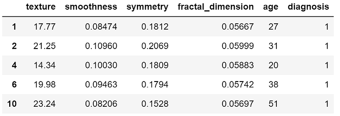
df.head()

We already dropped null values, but you can verify this visually by applying a heat map.

import matplotlib.pyplot as plt
import seaborn as sns
%matplotlib inline
# simple heat map showing where we are missing data
heat_map = sns.heatmap(df.isnull(), yticklabels = False, cbar = True, cmap = "PuRd", vmin = 0, vmax = 1)
plt.show()

So far, we have…

• Dropped categorical variables (id and name)
• Identified highly correlated predictor variables via VIF and dropped when VIF > 5
• Checked to see if we still have any nulls

We can now go on to build our logistic regression model!

Build the Model

Step 1: Split data into X and y

X = df.drop('diagnosis', axis = 1)
y = df['diagnosis']
X.head()

y.head()

Step 2: Split data into a train set and a test set

from sklearn.model_selection import train_test_split
X_train, X_test, y_train, y_test = train_test_split(X, y, test_size = 0.3, random_state = 101)

Step 3: Train and predict

from sklearn.linear_model import LogisticRegression
logreg = LogisticRegression()
logreg.fit(X_train, y_train)
y_predictions = logreg.predict(X_test)
y_predictions

where 1 indicates a patient having breast cancer and 0 indicates a patient not having breast cancer.

Evaluate the Model

Classification Report

from sklearn.metrics import classification_report
classification_report(y_test, y_predictions)

So, our model was able to predict 66% of relevant results (precision) and correctly classify 67% of all relevant results (recall).

Confusion Matrix

from sklearn.metrics import confusion_matrix
confusion_matrix(y_test, y_predictions)

• 150 women in test set
• Out of the 91 women predicted to not have breast cancer (diagnosis = 0), 14 women were incorrectly classified as not having breast cancer when they actually did. -> Type 1 Error
• Out of the 59 women predicted to have breast cancer (diagnosis = 1), 36 were incorrectly classified as having breast cancer when they did not. -> Type 2 Error

Conclusion

By removing the highly correlated independent variables (radius, perimeter, area, compactness, and concavity), we have increased the overall reliability of our regression results. On the other hand, though, our model performed much worse this time around (~90% accuracy -> ~66% accuracy).

Author Note

Thanks for reading! Please feel free to follow me on Medium and LinkedIn. I’d love to continue the conversation and hear your thoughts/suggestions.

-Mo